Simulation and Testing

Simulation

class pyrtl.simulation.Simulation(tracer=True, register_value_map={}, memory_value_map={}, default_value=0, block=None)

A class for simulating blocks of logic step by step.

A Simulation step works as follows:

1. Registers are updated:

   1. (If this is the first step) With the default values passed in to the Simulation during instantiation and/or any reset values specified in the individual registers.

   2. (Otherwise) With their next values calculated in the previous step (r logic nets).

2. The new values of these registers as well as the values of block inputs are propagated through the combinational logic.

3. Memory writes are performed (@ logic nets).

4. The current values of all wires are recorded in the trace.

5. The next values for the registers are saved, ready to be applied at the beginning of the next step.

Note that the register values saved in the trace after each simulation step are from before the register has latched in its newly calculated values, since that latching in occurs at the beginning of the next step.

In addition to the functions methods listed below, it is sometimes useful to reach into this class and access internal state directly. Of particular usefulness are:

• .tracer: stores the SimulationTrace in which results are stored

• .value: a map from every signal in the block to its current simulation value

• .regvalue: a map from register to its value on the next tick

• .memvalue: a map from memid to a dictionary of address: value

__init__(tracer=True, register_value_map={}, memory_value_map={}, default_value=0, block=None)

Creates a new circuit simulator.

Parameters:

• tracer (SimulationTrace) – Stores execution results. Defaults to a new SimulationTrace with no params passed to it. If None is passed, no tracer is instantiated (which is good for long running simulations). If the default (true) is passed, Simulation will create a new tracer automatically which can be referenced by the member variable .tracer

• register_value_map (dict[Register, int]) – Defines the initial value for the registers specified; overrides the registers’s reset_value.

• memory_value_map – Defines initial values for many addresses in a single or multiple memory. Format: {Memory: {address: Value}}. Memory is a memory block, address is the address of a value

• default_value (int) – The value that all unspecified registers and memories will initialize to (default 0). For registers, this is the value that will be used if the particular register doesn’t have a specified reset_value, and isn’t found in the register_value_map.

• block (Block) – the hardware block to be traced (which might be of type PostSynthBlock). Defaults to the working block

Warning: Simulation initializes some things when called with __init__(), so changing items in the block for Simulation will likely break the simulation.

inspect(w)

Get the value of a WireVector in the last simulation cycle.

Parameters:

w (str) – the name of the WireVector to inspect (passing in a WireVector instead of a name is deprecated)

Returns:

value of w in the current step of simulation

Will throw KeyError if w does not exist in the simulation.

Example:

sim.inspect('a') == 10  # returns value of wire 'a' at current step

inspect_mem(mem)

Get the values in a map during the current simulation cycle.

Parameters:

mem – the memory to inspect

Returns:

{address: value}

Note that this returns the current memory state. Modifying the dictonary will also modify the state in the simulator

step(provided_inputs)

Take the simulation forward one cycle.

Parameters:

provided_inputs – a dictionary mapping WireVectors to their values for this step

A step causes the block to be updated as follows, in order:

1. Registers are updated with their next values computed in the previous cycle

2. Block inputs and these new register values propagate through the combinational logic

3. Memories are updated

4. The next values of the registers are saved for use in step 1 of the next cycle.

All input wires must be in the provided_inputs in order for the simulation to accept these values.

Example: if we have inputs named a and x, we can call:

sim.step({'a': 1, 'x': 23})

to simulate a cycle with values 1 and 23 respectively.

step_multiple(provided_inputs={}, expected_outputs={}, nsteps=None, file=<_io.TextIOWrapper name='<stdout>' mode='w' encoding='utf-8'>, stop_after_first_error=False)

Take the simulation forward N cycles, based on the number of values for each input

Parameters:

• provided_inputs – a dictionary mapping WireVectors to their values for N steps

• expected_outputs – a dictionary mapping WireVectors to their expected values for N steps; use ? to indicate you don’t care what the value at that step is

• nsteps – number of steps to take (defaults to None, meaning step for each supplied input value)

• file – where to write the output (if there are unexpected outputs detected)

• stop_after_first_error – a boolean flag indicating whether to stop the simulation after encountering the first error (defaults to False)

All input wires must be in the provided_inputs in order for the simulation to accept these values. Additionally, the length of the array of provided values for each input must be the same.

When nsteps is specified, then it must be less than or equal to the number of values supplied for each input when provided_inputs is non-empty. When provided_inputs is empty (which may be a legitimate case for a design that takes no inputs), then nsteps will be used. When nsteps is not specified, then the simulation will take the number of steps equal to the number of values supplied for each input.

Example: if we have inputs named a and b and output o, we can call:

sim.step_multiple({'a': [0,1], 'b': [23,32]}, {'o': [42, 43]})

to simulate 2 cycles, where in the first cycle a and b take on 0 and 23, respectively, and o is expected to have the value 42, and in the second cycle a and b take on 1 and 32, respectively, and o is expected to have the value 43.

If your values are all single digit, you can also specify them in a single string, e.g.:

sim.step_multiple({'a': '01', 'b': '01'})

will simulate 2 cycles, with a and b taking on 0 and 0, respectively, on the first cycle and 1 and 1, respectively, on the second cycle.

Example: if the design had no inputs, like so:

a = pyrtl.Register(8)
b = pyrtl.Output(8, 'b')

a.next <<= a + 1
b <<= a

sim = pyrtl.Simulation()
sim.step_multiple(nsteps=3)

Using sim.step_multiple(nsteps=3) simulates 3 cycles, after which we would expect the value of b to be 2.

Fast (JIT to Python) Simulation

class pyrtl.simulation.FastSimulation(register_value_map={}, memory_value_map={}, default_value=0, tracer=True, block=None, code_file=None)

A class for running JIT-to-python implementations of blocks.

A Simulation step works as follows:

1. Registers are updated:

   1. (If this is the first step) With the default values passed in to the Simulation during instantiation and/or any reset values specified in the individual registers.

   2. (Otherwise) With their next values calculated in the previous step (r logic nets).

2. The new values of these registers as well as the values of block inputs are propagated through the combinational logic.

3. Memory writes are performed (@ logic nets).

4. The current values of all wires are recorded in the trace.

5. The next values for the registers are saved, ready to be applied at the beginning of the next step.

Note that the register values saved in the trace after each simulation step are from before the register has latched in its newly calculated values, since that latching in occurs at the beginning of the next step.

__init__(register_value_map={}, memory_value_map={}, default_value=0, tracer=True, block=None, code_file=None)

Instantiates a Fast Simulation instance.

The interface for FastSimulation and Simulation should be almost identical. In addition to the Simulation arguments, FastSimulation additionally takes:

Parameters:

code_file – The file in which to store a copy of the generated Python code. Defaults to no code being stored.

Look at Simulation.__init__() for descriptions for the other parameters.

This builds the Fast Simulation compiled Python code, so all changes to the circuit after calling this function will not be reflected in the simulation.

inspect(w)

Get the value of a WireVector in the last simulation cycle.

Parameters:

w (str) – the name of the WireVector to inspect (passing in a WireVector instead of a name is deprecated)

Returns:

value of w in the current step of simulation

Will throw KeyError if w is not being tracked in the simulation.

inspect_mem(mem)

Get the values in a map during the current simulation cycle.

Parameters:

mem – the memory to inspect

Returns:

{address: value}

Note that this returns the current memory state. Modifying the dictonary will also modify the state in the simulator

step(provided_inputs)

Run the simulation for a cycle.

Parameters:

provided_inputs – a dictionary mapping WireVectors (or their names) to their values for this step (eg: {wire: 3, “wire_name”: 17})

A step causes the block to be updated as follows, in order:

1. Registers are updated with their next values computed in the previous cycle

2. Block inputs and these new register values propagate through the combinational logic

3. Memories are updated

4. The next values of the registers are saved for use in step 1 of the next cycle.

step_multiple(provided_inputs={}, expected_outputs={}, nsteps=None, file=<_io.TextIOWrapper name='<stdout>' mode='w' encoding='utf-8'>, stop_after_first_error=False)

Take the simulation forward N cycles, where N is the number of

values for each provided input.

Parameters:

• provided_inputs – a dictionary mapping WireVectors to their values for N steps

• expected_outputs – a dictionary mapping WireVectors to their expected values for N steps; use ? to indicate you don’t care what the value at that step is

• nsteps – number of steps to take (defaults to None, meaning step for each supplied input value)

• file – where to write the output (if there are unexpected outputs detected)

• stop_after_first_error – a boolean flag indicating whether to stop the simulation after the step where the first errors are encountered (defaults to False)

All input wires must be in the provided_inputs in order for the simulation to accept these values. Additionally, the length of the array of provided values for each input must be the same.

When nsteps is specified, then it must be less than or equal to the number of values supplied for each input when provided_inputs is non-empty. When provided_inputs is empty (which may be a legitimate case for a design that takes no inputs), then nsteps will be used. When nsteps is not specified, then the simulation will take the number of steps equal to the number of values supplied for each input.

Example: if we have inputs named a and b and output o, we can call:

sim.step_multiple({'a': [0,1], 'b': [23,32]}, {'o': [42, 43]})

to simulate 2 cycles, where in the first cycle a and b take on 0 and 23, respectively, and o is expected to have the value 42, and in the second cycle a and b take on 1 and 32, respectively, and o is expected to have the value 43.

If your values are all single digit, you can also specify them in a single string, e.g.:

sim.step_multiple({'a': '01', 'b': '01'})

will simulate 2 cycles, with a and b taking on 0 and 0, respectively, on the first cycle and 1 and 1, respectively, on the second cycle.

Example: if the design had no inputs, like so:

a = pyrtl.Register(8)
b = pyrtl.Output(8, 'b')

a.next <<= a + 1
b <<= a

sim = pyrtl.Simulation()
sim.step_multiple(nsteps=3)

Using sim.step_multiple(nsteps=3) simulates 3 cycles, after which we would expect the value of b to be 2.

Compiled (JIT to C) Simulation

class pyrtl.compilesim.CompiledSimulation(tracer=True, register_value_map={}, memory_value_map={}, default_value=0, block=None)

Simulate a block, compiling to C for efficiency.

This module provides significant speed improvements over FastSimulation, at the cost of somewhat longer setup time. Generally this will do better than FastSimulation for simulations requiring over 1000 steps. It is not built to be a debugging tool, though it may help with debugging. Note that only Input and Output wires can be traced using CompiledSimulation. This code is still experimental, but has been used on designs of significant scale to good effect.

In order to use this, you need:

• A 64-bit processor

• GCC (tested on version 4.8.4)

• A 64-bit build of Python

If using the multiplication operand, only some architectures are supported:

• x86-64 / amd64

• arm64 / aarch64

• mips64 (untested)

default_value is currently only implemented for registers, not memories.

A Simulation step works as follows:

1. Registers are updated:

   1. (If this is the first step) With the default values passed in to the Simulation during instantiation and/or any reset values specified in the individual registers.

   2. (Otherwise) With their next values calculated in the previous step (r logic nets).

2. The new values of these registers as well as the values of block inputs are propagated through the combinational logic.

3. Memory writes are performed (@ logic nets).

4. The current values of all wires are recorded in the trace.

5. The next values for the registers are saved, ready to be applied at the beginning of the next step.

Note that the register values saved in the trace after each simulation step are from before the register has latched in its newly calculated values, since that latching in occurs at the beginning of the next step.

__init__(tracer=True, register_value_map={}, memory_value_map={}, default_value=0, block=None)

inspect(w)

Get the latest value of the wire given, if possible.

inspect_mem(mem)

Get a view into the contents of a MemBlock.

run(inputs)

Run many steps of the simulation.

Parameters:

inputs – A list of input mappings for each step; its length is the number of steps to be executed.

step(inputs)

Run one step of the simulation.

Parameters:

inputs – A mapping from input names to the values for the step.

A step causes the block to be updated as follows, in order:

1. Registers are updated with their next values computed in the previous cycle

2. Block inputs and these new register values propagate through the combinational logic

3. Memories are updated

4. The next values of the registers are saved for use in step 1 of the next cycle.

step_multiple(provided_inputs={}, expected_outputs={}, nsteps=None, file=<_io.TextIOWrapper name='<stdout>' mode='w' encoding='utf-8'>, stop_after_first_error=False)

Take the simulation forward N cycles, where N is the number of values

for each provided input.

Parameters:

• provided_inputs – a dictionary mapping wirevectors to their values for N steps

• expected_outputs – a dictionary mapping wirevectors to their expected values for N steps; use ? to indicate you don’t care what the value at that step is

• nsteps – number of steps to take (defaults to None, meaning step for each supplied input value)

• file – where to write the output (if there are unexpected outputs detected)

• stop_after_first_error – a boolean flag indicating whether to stop the simulation after the step where the first errors are encountered (defaults to False)

All input wires must be in the provided_inputs in order for the simulation to accept these values. Additionally, the length of the array of provided values for each input must be the same.

When nsteps is specified, then it must be less than or equal to the number of values supplied for each input when provided_inputs is non-empty. When provided_inputs is empty (which may be a legitimate case for a design that takes no inputs), then nsteps will be used. When nsteps is not specified, then the simulation will take the number of steps equal to the number of values supplied for each input.

Example: if we have inputs named a and b and output o, we can call:

sim.step_multiple({'a': [0,1], 'b': [23,32]}, {'o': [42, 43]})

to simulate 2 cycles, where in the first cycle a and b take on 0 and 23, respectively, and o is expected to have the value 42, and in the second cycle a and b take on 1 and 32, respectively, and o is expected to have the value 43.

If your values are all single digit, you can also specify them in a single string, e.g.:

sim.step_multiple({'a': '01', 'b': '01'})

will simulate 2 cycles, with a and b taking on 0 and 0, respectively, on the first cycle and 1 and 1, respectively, on the second cycle.

Example: if the design had no inputs, like so:

a = pyrtl.Register(8)
b = pyrtl.Output(8, 'b')

a.next <<= a + 1
b <<= a

sim = pyrtl.Simulation()
sim.step_multiple(nsteps=3)

Using sim.step_multiple(nsteps=3) simulates 3 cycles, after which we would expect the value of b to be 2.

Simulation Trace

class pyrtl.simulation.SimulationTrace(wires_to_track=None, block=None)

Storage and presentation of simulation waveforms.

__init__(wires_to_track=None, block=None)

Creates a new Simulation Trace

Parameters:

• wires_to_track – The wires that the tracer should track. If unspecified, will track all explicitly-named wires. If set to 'all', will track all wires, including internal wires.

• block – Block containing logic to trace

add_fast_step(fastsim)

Add the fastsim context to the trace.

add_step(value_map)

Add the values in value_map to the end of the trace.

print_perf_counters(*trace_names, file=<_io.TextIOWrapper name='<stdout>' mode='w' encoding='utf-8'>)

Print performance counter statistics for trace_names.

Parameters:

• trace_names (str) – List of trace names. Each trace must be a single-bit wire.

• file – The place to write output, defaults to stdout.

This function prints the number of cycles where each trace’s value is one. This is useful for counting the number of times important events occur in a simulation, such as cache misses and branch mispredictions.

print_trace(file=<_io.TextIOWrapper name='<stdout>' mode='w' encoding='utf-8'>, base=10, compact=False)

Prints a list of wires and their current values.

Parameters:

• base (int) – the base the values are to be printed in

• compact (bool) – whether to omit spaces in output lines

print_vcd(file=<_io.TextIOWrapper name='<stdout>' mode='w' encoding='utf-8'>, include_clock=False)

Print the trace out as a VCD File for use in other tools.

Parameters:

• file – file to open and output vcd dump to.

• include_clock – boolean specifying if the implicit clk should be included.

Dumps the current trace to file as a value change dump file. The file parameter defaults to stdout and the include_clock defaults to False.

Examples:

sim_trace.print_vcd()
sim_trace.print_vcd("my_waveform.vcd", include_clock=True)

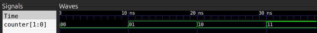
render_trace(trace_list=None, file=<_io.TextIOWrapper name='<stdout>' mode='w' encoding='utf-8'>, renderer=<pyrtl.simulation.WaveRenderer object>, symbol_len=None, repr_func=<built-in function hex>, repr_per_name={}, segment_size=1)

Render the trace to a file using unicode and ASCII escape sequences.

Parameters:

• trace_list (list[str]) – A list of signal names to be output in the specified order.

• file – The place to write output, default to stdout.

• renderer (WaveRenderer) – An object that translates traces into output bytes.

• symbol_len (int) – The “length” of each rendered value in characters. If None, the length will be automatically set such that the largest represented value fits.

• repr_func – Function to use for representing each value in the trace; examples are hex, oct, bin, and str (for decimal), or the function returned by enum_name(). Defaults to ‘hex’.

• repr_per_name – Map from signal name to a function that takes in the signal’s value and returns a user-defined representation. If a signal name is not found in the map, the argument repr_func will be used instead.

• segment_size (int) – Traces are broken in the segments of this number of cycles.

The resulting output can be viewed directly on the terminal or looked at with more or less -R which both should handle the ASCII escape sequences used in rendering.

Wave Renderer

class pyrtl.simulation.WaveRenderer(constants)

Render a SimulationTrace to the terminal.

See examples/renderer-demo.py, which renders traces with various options. You can choose a default renderer by exporting the PYRTL_RENDERER environment variable. See the documentation for subclasses of RendererConstants.

__init__(constants)

Instantiate a WaveRenderer.

Parameters:

constants – Subclass of RendererConstants that specifies the ASCII/Unicode characters to use for rendering waveforms.

pyrtl.simulation.enum_name(EnumClass)

Returns a function that returns the name of an enum value as a string.

Use enum_name as a repr_func or repr_per_name for SimulationTrace.render_trace() to display enum names, instead of their numeric value, in traces. Example:

class State(enum.IntEnum):
    FOO = 0
    BAR = 1
state = Input(name='state', bitwidth=1)
sim = Simulation()
sim.step_multiple({'state': [State.FOO, State.BAR]})

# Generates a trace like:
#      │0  │1
#
# state FOO│BAR
sim.tracer.render_trace(repr_per_name={'state': enum_name(State)})

Parameters:

EnumClass (type) – enum to convert. This is the enum class, like State, not an enum value, like State.FOO or 1.

Return type:

Callable[[int], str]

Returns:

A function that accepts an enum value, like State.FOO or 1, and returns the value’s name as a string, like 'FOO'.

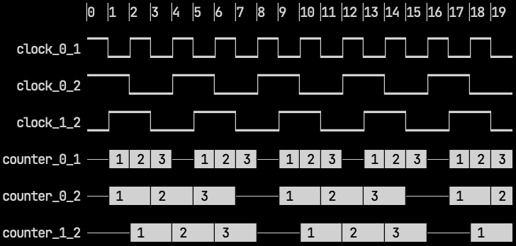
class pyrtl.simulation.PowerlineRendererConstants

Bases: Utf8RendererConstants

Powerline renderer constants. Font must include powerline glyphs.

This render is closest to a traditional logic analyzer. Single-bit WireVectors are rendered as square waveforms, with vertical rising and falling edges. Multi-bit WireVector values are rendered in reverse-video hexagons.

This renderer requires a terminal font that supports Powerline glyphs

Enable this renderer by default by setting the PYRTL_RENDERER environment variable to powerline.

class pyrtl.simulation.Utf8RendererConstants

Bases: RendererConstants

UTF-8 renderer constants. These should work in most terminals.

Single-bit WireVectors are rendered as square waveforms, with vertical rising and falling edges. Multi-bit WireVector values are rendered in reverse-video rectangles.

This is the default renderer on non-Windows platforms.

Enable this renderer by default by setting the PYRTL_RENDERER environment variable to utf-8.

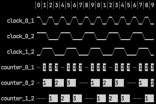
class pyrtl.simulation.Utf8AltRendererConstants

Bases: RendererConstants

Alternative UTF-8 renderer constants.

Single-bit WireVectors are rendered as waveforms with sloped rising and falling edges. Multi-bit WireVector values are rendered in reverse-video rectangles.

Compared to Utf8RendererConstants, this renderer is more compact because it uses one character between cycles instead of two.

Enable this renderer by default by setting the PYRTL_RENDERER environment variable to utf-8-alt.

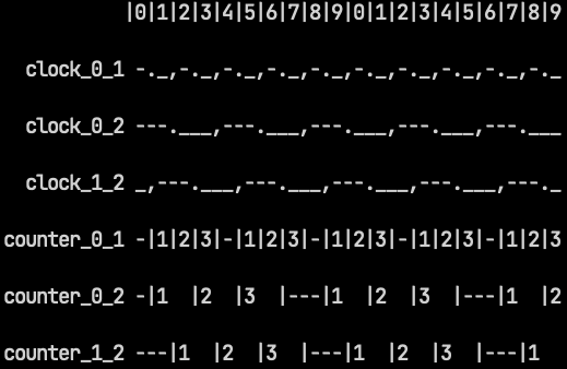
class pyrtl.simulation.Cp437RendererConstants

Bases: RendererConstants

Code page 437 renderer constants (for windows cmd compatibility).

Single-bit WireVectors are rendered as square waveforms, with vertical rising and falling edges. Multi-bit WireVector values are rendered between vertical bars.

Code page 437 is also known as 8-bit ASCII. This is the default renderer on Windows platforms.

Compared to Utf8RendererConstants, this renderer is more compact because it uses one character between cycles instead of two, but the wire names are vertically aligned at the bottom of each waveform.

Enable this renderer by default by setting the PYRTL_RENDERER environment variable to cp437.

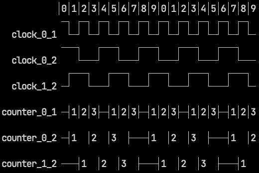
class pyrtl.simulation.AsciiRendererConstants

Bases: RendererConstants

7-bit ASCII renderer constants. These should work anywhere.

Single-bit WireVectors are rendered as waveforms with sloped rising and falling edges. Multi-bit WireVector values are rendered between vertical bars.

Enable this renderer by default by setting the PYRTL_RENDERER environment variable to ascii.